TensorFlow

Use CnosDB and TensorFlow for time series prediction

From three-body motion to Sunspot Change prediction

Introduction

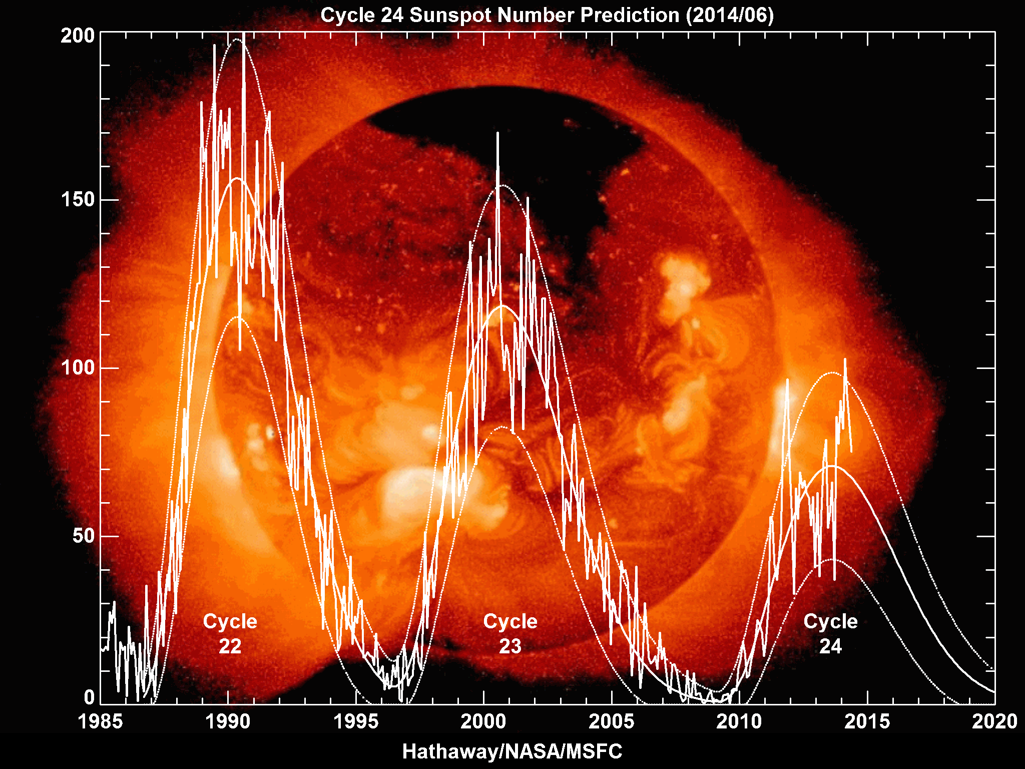
Sunspots are solar activity that occurs in the photosphere of the sun and usually appear in groups. Predicting sunspot changes is one of the most active areas of space weather research.

Sunspot observations last for a long time. Long-term data accumulation is conducive to mining the law of sunspot variation. The long-term observation shows that the sunspot number and area change show obvious periodicity, and the period is irregular, roughly ranging from 9 to 13 years, the average period is about 11 years, and the peak value of the sunspot number and area change is not constant.

The latest data show that the number and area of sunspots have declined significantly in recent years.

Since the intensity of sunspot activity has a profound impact on Earth, it is particularly important to detect sunspot activity. Physics-based models, such as dynamical models, and statistical models, such as autoregressive moving averages, have been widely used to detect sunspot activity. In order to capture the nonlinear relationship in sunspot time series more efficiently, machine learning methods are introduced.

It is worth mentioning that neural networks in machine learning are better at mining nonlinear relationships in data.

Therefore, this article will introduce how to use the time series database 'CnosDB' to store the sunspot change data and further use TensorFlow to implement the '1DConv+LSTM' network to predict the sunspot number change.

Introduction to the Sunspot Change Observation dataset

The sunspot dataset used in this paper was released by the SILSO website version 2.0. (WDC-SILSO, Royal Observatory of Belgium, Brussels,http://sidc.be/silso/datafiles)

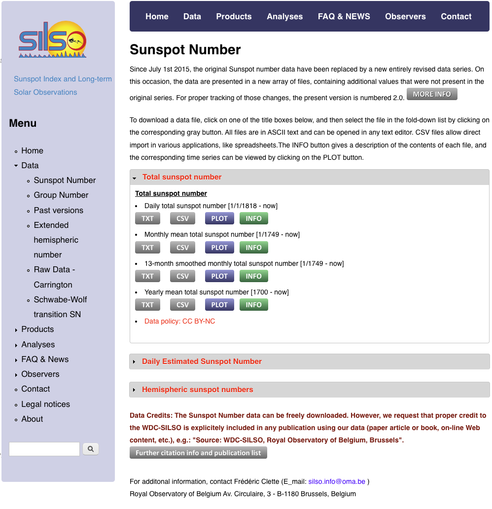
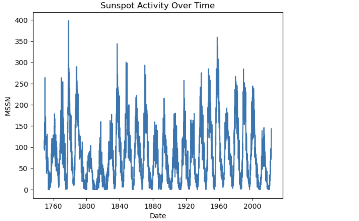
We mainly analyze and explore the changes of the monthly mean sunspot number (MSSN) from 1749 to 2023.

Import Data to CnosDB

Download MSSN data SN_m_tot_V2.0.csv（https://www.sidc.be/SILSO/INFO/snmtotcsv.php）.

Here is the official description of the CSV file:

Filename: SN_m_tot_V2.0.csv
Format: Comma Separated values (adapted for import in spreadsheets)
The separator is the semicolon ';'.

Contents:
Column 1-2: Gregorian calendar date
- Year
- Month
Column 3: Date in fraction of year.
Column 4: Monthly mean total sunspot number.
Column 5: Monthly mean standard deviation of the input sunspot numbers.
Column 6: Number of observations used to compute the monthly mean total sunspot number.
Column 7: Definitive/provisional marker. '1' indicates that the value is definitive. '0' indicates that the value is still provisional.

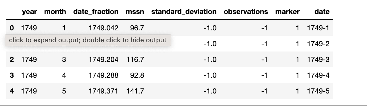
We use pandas for file loading and previewing.

import pandas as pd

df = pd.read_csv("SN_m_tot_V2.0.csv", sep=";", header=None)
df.columns = ["year", "month", "date_fraction", "mssn", "standard_deviation", "observations", "marker"]

# convert year and month to strings
df["year"] = df["year"].astype(str)
df["month"] = df["month"].astype(str)

# concatenate year and month
df["date"] = df["year"] + "-" + df["month"]

df.head()

import matplotlib.pyplot as plt

df["Date"] = pd.to_datetime(df["date"], format="%Y-%m")
plt.plot(df["Date"], df["mssn"])
plt.xlabel("Date")
plt.ylabel("MSSN")
plt.title("Sunspot Activity Over Time")
plt.show()

Use TSDB CnosDB to store MSSN data

CnosDB（An Open Source Distributed Time Series Database with high performance, high compression ratio and high usability.）

Official Website: http://www.cnosdb.com
Github Repo: https://github.com/cnosdb/cnosdb

Notice: We suppose the you have the ability to deploy and use CnosDB. You can get more information through https://docs.cnosdb.com/）

Use Docker to start CnosDB service in command line, enter the container and use the CnosDB CLI to use CnosDB:

(base) root@ecs-django-dev:~# docker run --restart=always --name cnosdb -d --env cpu=2 --env memory=4 -p 8902:8902 cnosdb/cnosdb:v2.0.2.1-beta

(base) root@ecs-django-dev:~# docker exec -it cnosdb sh sh
# cnosdb-cli
CnosDB CLI v2.3.0
Input arguments: Args { host: "localhost", port: 8902, user: "cnosdb", password: None, database: "public", target_partitions: None, data_path: None, file: [], rc: None, format: Table, quiet: false }

To simplify the analysis, we only need to store the observation time and the number of sunspots in the dataset. Therefore, we concatenate the year (Col 0) and month (Col 1) as the observation time (date, string type), and the monthly mean sunspot number (Col 3) can be stored directly without processing.

We can create a 'sunspot' table in CnosDB CLI using SQL to store the MSSN dataset.

public ❯ CREATE TABLE sunspot (
date STRING,
mssn DOUBLE,
);
Query took 0.002 seconds.

public ❯ SHOW TABLES;
+---------+
| Table   |
+---------+
| sunspot |
+---------+
Query took 0.001 seconds.

public ❯ SELECT * FROM sunspot;
+------+------+------+
| time | date | mssn |
+------+------+------+
+------+------+------+
Query took 0.002 seconds.

Use CnosDB Python Connector to Connect and Use CnosDB Database

Github Repo: https://github.com/cnosdb/cnosdb-client-python

# install Python Connector
pip install -U cnos-connector

from cnosdb_connector import connect

conn = connect(url="http://127.0.0.1:8902/", user="root", password="")
cursor = conn.cursor()

If you are not familiar with CnosDB CLI, We can use Python Connector to create a data table.

# create tf_demo database
conn.create_database("tf_demo")
# 使用 tf_demo database
conn.switch_database("tf_demo")
print(conn.list_database())

cursor.execute("CREATE TABLE sunspot (date STRING, mssn DOUBLE,);")
print(conn.list_table())

Outputs are as follows, the default database of CnosDB included.

[{'Database': 'tf_demo'}, {'Database': 'usage_schema'}, {'Database': 'public'}]
[{'Table': 'sunspot'}]

Write the dataframe of pandas to CnosDB.

### df is the dataframe of pandas, "sunspot" is the table name of CnosDB, ['date', 'mssn'] are the name of columns to be written.
### If you write a column that does not contain a time column, it will be automatically generated based on the current time
conn.write_dataframe(df, "sunspot", ['date', 'mssn'])

CnoDB reads the data and uses TensorFlow to reproduce the 1DConv+LSTM network to predict sunspot changes

References: 程术, 石耀霖, and 张怀. "基于神经网络预测太阳黑子变化." (2022).

Use CnosDB to Read Data

df = pd.read_sql("select * from sunspot;", conn)

print(df.head())

Divide the data into training set and test set

import numpy as np
# Convert the data values to numpy for better and faster processing
time_index = np.array(df['date'])
data = np.array(df['mssn'])

# ratio to split the data
SPLIT_RATIO = 0.8

# Dividing into train-test split
split_index = int(SPLIT_RATIO * data.shape[0])

# Train-Test Split
train_data = data[:split_index]
train_time = time_index[:split_index]
test_data = data[split_index:]
test_time = time_index[split_index:]

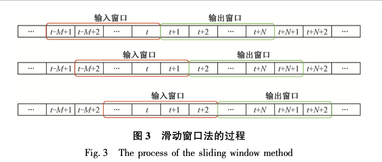
Use the Sliding Window Method to Construct the Training Data

import tensorflow as tf

## required parameters
WINDOW_SIZE = 60
BATCH_SIZE = 32
SHUFFLE_BUFFER = 1000

## function to create the input features
def ts_data_generator(data, window_size, batch_size, shuffle_buffer):
'''
Utility function for time series data generation in batches
'''
ts_data = tf.data.Dataset.from_tensor_slices(data)
ts_data = ts_data.window(window_size + 1, shift=1, drop_remainder=True)
ts_data = ts_data.flat_map(lambda window: window.batch(window_size + 1))
ts_data = ts_data.shuffle(shuffle_buffer).map(lambda window: (window[:-1], window[-1]))
ts_data = ts_data.batch(batch_size).prefetch(1)
return ts_data# Expanding data into tensors


# Expanding data into tensors
tensor_train_data = tf.expand_dims(train_data, axis=-1)
tensor_test_data = tf.expand_dims(test_data, axis=-1)

## generate input and output features for training and testing set
tensor_train_dataset = ts_data_generator(tensor_train_data, WINDOW_SIZE, BATCH_SIZE, SHUFFLE_BUFFER)
tensor_test_dataset = ts_data_generator(tensor_test_data, WINDOW_SIZE, BATCH_SIZE, SHUFFLE_BUFFER)

Use the tf.keras module to Define the 1DConv+LSTM Neural Network Model

model = tf.keras.models.Sequential([
tf.keras.layers.Conv1D(filters=128, kernel_size=3, strides=1, input_shape=[None, 1]),
tf.keras.layers.MaxPool1D(pool_size=2, strides=1),
tf.keras.layers.LSTM(128, return_sequences=True),
tf.keras.layers.LSTM(64, return_sequences=True),
tf.keras.layers.Dense(132, activation="relu"),
tf.keras.layers.Dense(1)])

## compile neural network model
optimizer = tf.keras.optimizers.Adam(learning_rate=1e-3)
model.compile(loss="mse",
optimizer=optimizer,
metrics=["mae"])
## training neural network model
history = model.fit(tensor_train_dataset, epochs=20, validation_data=tensor_test_dataset)

# summarize history for loss
plt.plot(history.history['loss'])
plt.plot(history.history['val_loss'])
plt.title('model loss')
plt.ylabel('loss')
plt.xlabel('epoch')
plt.legend(['train', 'test'], loc='upper left')
plt.show()

Predict the MSSN using the trained model

def model_forecast(model, data, window_size):
ds = tf.data.Dataset.from_tensor_slices(data)
ds = ds.window(window_size, shift=1, drop_remainder=True)
ds = ds.flat_map(lambda w: w.batch(window_size))
ds = ds.batch(32).prefetch(1)
forecast = model.predict(ds)
return forecast

rnn_forecast = model_forecast(model, data[..., np.newaxis], WINDOW_SIZE)
rnn_forecast = rnn_forecast[split_index - WINDOW_SIZE:-1, -1, 0]
# Overall Error
error = tf.keras.metrics.mean_absolute_error(test_data, rnn_forecast).numpy()
print(error)

101/101 [==============================] - 2s 18ms/step
24.676455

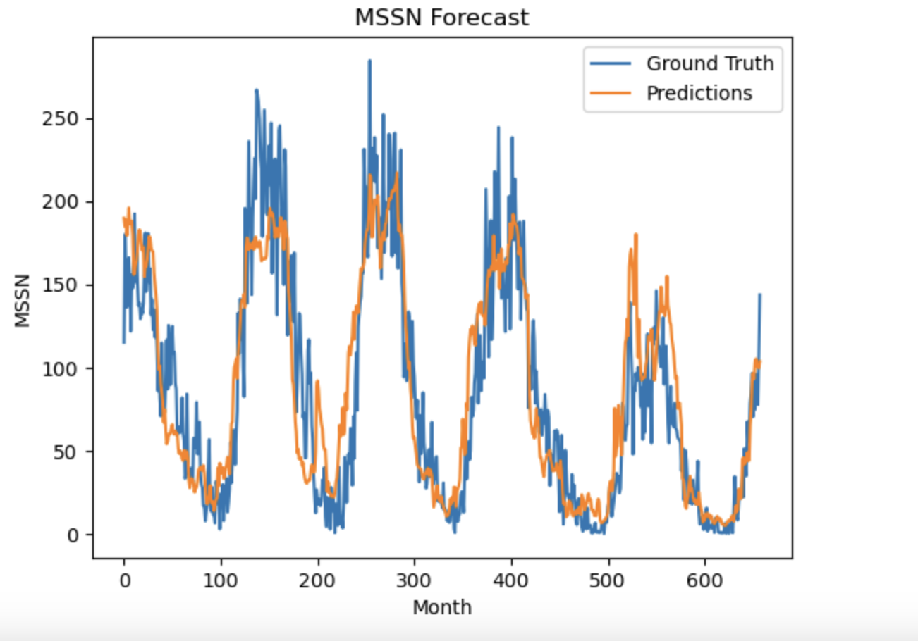
Visualization of the results compared to the ground truth

plt.plot(test_data)
plt.plot(rnn_forecast)
plt.title('MSSN Forecast')
plt.ylabel('MSSN')
plt.xlabel('Month')
plt.legend(['Ground Truth', 'Predictions'], loc='upper right')
plt.show()

TensorFlow​

Use CnosDB and TensorFlow for time series prediction​

From three-body motion to Sunspot Change prediction​

Introduction​

Introduction to the Sunspot Change Observation dataset​

Import Data to CnosDB​

Use TSDB CnosDB to store MSSN data​

Use CnosDB Python Connector to Connect and Use CnosDB Database​

CnoDB reads the data and uses TensorFlow to reproduce the 1DConv+LSTM network to predict sunspot changes​

Use CnosDB to Read Data​

Divide the data into training set and test set​

Use the Sliding Window Method to Construct the Training Data​

Use the tf.keras module to Define the 1DConv+LSTM Neural Network Model​

Predict the MSSN using the trained model​

Visualization of the results compared to the ground truth​